
Critical Learning Periods in Deep Networks
Why the first epochs matter the most…

Empirical demonstration of the existence of critical learning periods in both artificial and biological system (from [1])
What are Critical Learning Periods?
To understand critical learning periods within deep learning, it is helpful to first look at a related analogy to biological systems. Within humans and animals, critical periods are defined as times of early post-natal (i.e., after birth) development, during which impairments to learning (e.g., sensory deficits) can lead to permanent impairment of one’s skills [5]. For example, vision impairments at a young age—a critical period for the development of one’s eyesight—often lead to problems like amblyopia in adult humans.
Although I am far from a biological expert (in fact, I haven’t taken a biology class since high school), this concept of critical learning periods is still curiously relevant to deep learning, as the same behavior is exhibited within the learning process for neural networks. If a neural network is subjected to some impairment (e.g., only shown blurry images or not regularized properly) during the early phase of learning, the resulting network (after training is fully complete) will generalize more poorly relative to a network that never received such an early learning impairment, even given an unlimited training budget. Recovering from this early learning impairment is not possible.
In analyzing this curious behavior, researchers have found that neural network training seems to progress in two phases. During the first phase—the critical period that is sensitive to learning deficits—the network memorizes the data and passes through a bottleneck in the optimization landscape, eventually finding a more well-behaved region within which convergence can be achieved. From here, the network goes through a forgetting process and learns generalizable features rather than memorizing the data. In this phase, the network exists within a region of the loss landscape in which many equally-performant local optima exist, and eventually converges to one of these solutions.
Critical learning periods are fundamental to our understanding of deep learning as a whole. Within this overview, I will embrace the fundamental nature of the topic by first overviewing basic components of the neural network learning process. Given this background, my hope is that the resulting overview of critical learning periods will provide a more nuanced perspective that reveals the true complexity of training deep networks.
Background Information
Within this section, I will overview fundamental concepts within the training of deep networks. Such basic ideas are pivotal to understanding both the general learning process for neural networks and critical periods during learning. The overviews within this section are quite broad and may take time to truly grasp, so I provide further links for those who need more depth.
Neural Network Training
Neural network training is a fundamental aspect of deep learning. Covering the full depth of this topic is beyond the scope of this overview. However, to understand critical learning periods, one must have at least a basic grasp of the training procedure for neural networks.
The goal of neural network training is—starting from a neural network with randomly-initialized weights—to learn a set of parameters that allow the neural network to accurately produce a desired output given some input. Such input and output can take many forms—key points predicted on an image, a classification of text, object detections in a video, and more. Additionally, the neural network architecture oftentimes changes depending on the type of input data and problem being solved. Despite the variance in neural network definitions and applications, however, the basic concepts of model training remain (more or less) the same.
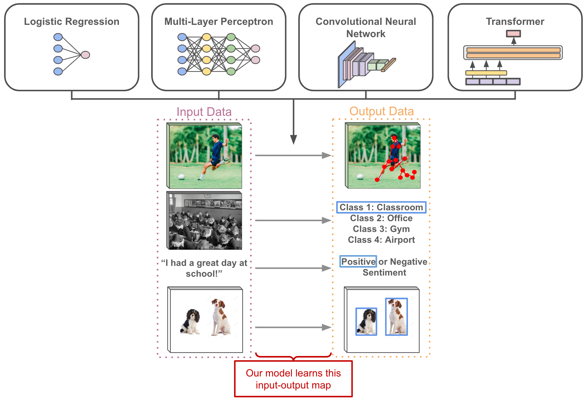
Depiction of the input-output map learned by neural networks in different problem domains
To learn this map between input and desired output, we need a (preferably large) training dataset of input-output pairs. Why? So that we can:
Make predictions on the data
See how the model’s predictions compare to the desired output
Update the model’s parameters to make predictions better
This process of updating the model’s parameters over training data to better match known labels is the crux of the learning process. For deep networks, this learning process is performed for several epochs, defined as full passes through the training dataset.
To determine the quality of model predictions, we define a loss function. The goal of training is to minimize this loss function, thus maximizing the quality of model predictions over training data. Because the loss function is typically chosen such that it is differentiable, we can differentiate the loss with respect to each parameter in the model and use stochastic gradient descent (SGD) to generate updates to model parameters. At a high level, SGD simply:
Computes the gradient of the loss function
Uses the chain rule of calculus to compute the gradient of the loss with respect to every parameter within the model
Subtracts the gradient, scaled by a learning rate, from each parameter
Although a bit complicated to understand in detail, SGD at an intuitive level is quite simple—each iteration just determines the direction that model parameters should be updated to decrease the loss and takes a small step in this direction. We perform optimization over the network’s parameters to minimize training loss. See below for a schematic depiction of this process, where the learning rate setting controls the size of each SGD step.
Minimization of the Training Loss with Different Learning Rates
In summary, the neural network training process proceeds for several epochs, each of which performs many iterations of SGD—typically using a mini-batch of several data examples at a time—over the training data. Over the course of training, the neural network’s loss over the training dataset becomes smaller and smaller, resulting in a model that fits the training data well and (hopefully) generalizes—meaning that it also performs well—to unseen testing data.

Basic Illustration of the Steps within a Neural Network Training Iteration
See the figure above for a high-level depiction of the neural network training process. There are many more details that go into neural network training, but the purpose of this overview is to understand critical learning periods, not to take a deep dive into neural network training. Thus, I provide below some links to useful articles that can be used to understand key neural network training concepts in greater detail for the interested reader.
SGD (and Other Optimization Algorithms) [blog]
Basic Neural Network Training in PyTorch [notebook]
What is generalization? [blog]
Regularization
Neural network training performs updates that minimize the loss over a training dataset. However, our goal in training this neural network is not just to achieve good performance over the training set. We also want the network to perform well on unseen testing data when it is deployed into the real world. A model that performs well on such unseen data is said to generalize well.
Minimizing loss on the training data does not guarantee that a model will generalize. For example, a model could just “memorize” each training example, thus preventing it from learning generalizable patterns that can be applied to unseen data. To ensure good generalization, deep learning practitioners typically utilize regularization techniques. Many such techniques exist, but the most relevant for the purposes of this post are weight decay and data augmentation.
Weight decay is a technique that is commonly applied to the training of machine learning models (even beyond neural networks). The idea is simple. During training, adjust your loss function to penalize the model for learning parameters with large magnitude. Then, optimizing the loss function becomes a joint goal of (i) minimizing loss over the training set and (ii) making network parameters low in magnitude. The strength of weight decay during training can be adjusted to find different tradeoffs between these two goals—it is another hyperparameter of the learning process that can be tweaked/modified (similar to the learning rate). To learn more, I suggest reading this article.
Data augmentation takes many different forms depending on the domain and setting in which it is being applied. But, the fundamental idea behind data augmentation remains constant—each time your model encounters some data during training, one should randomly change the data a little bit in a way that still preserves the data’s output label. Thus, your model never sees the same data example twice. Rather, the data is always slightly perturbed, preventing the model from simply memorizing examples from the training set. Although data augmentation can take many different forms, numerous survey papers and explanations exist that can be used to better understand these techniques.
Training, Pre-Training, and Fine-Tuning
Beyond the basic neural network training framework presented within this section, one will also frequently encounter the ideas of pre-training and fine-tuning for deep networks. All of these methods follow the same learning process outlined above—pre-training and fine-tuning are just terms that refer to a specific, slightly-modified setup for the same training process.
Pre-training typically refers to training a model from scratch (i.e., random initialization) over a very large dataset. Although such training over large pre-training datasets is computationally expensive, model weights learned from pre-training can be very useful, as they contain patterns that have been learned from raining over a lot of data that may generalize elsewhere (e.g., learning how to detect edges, understanding shapes/textures, etc.).
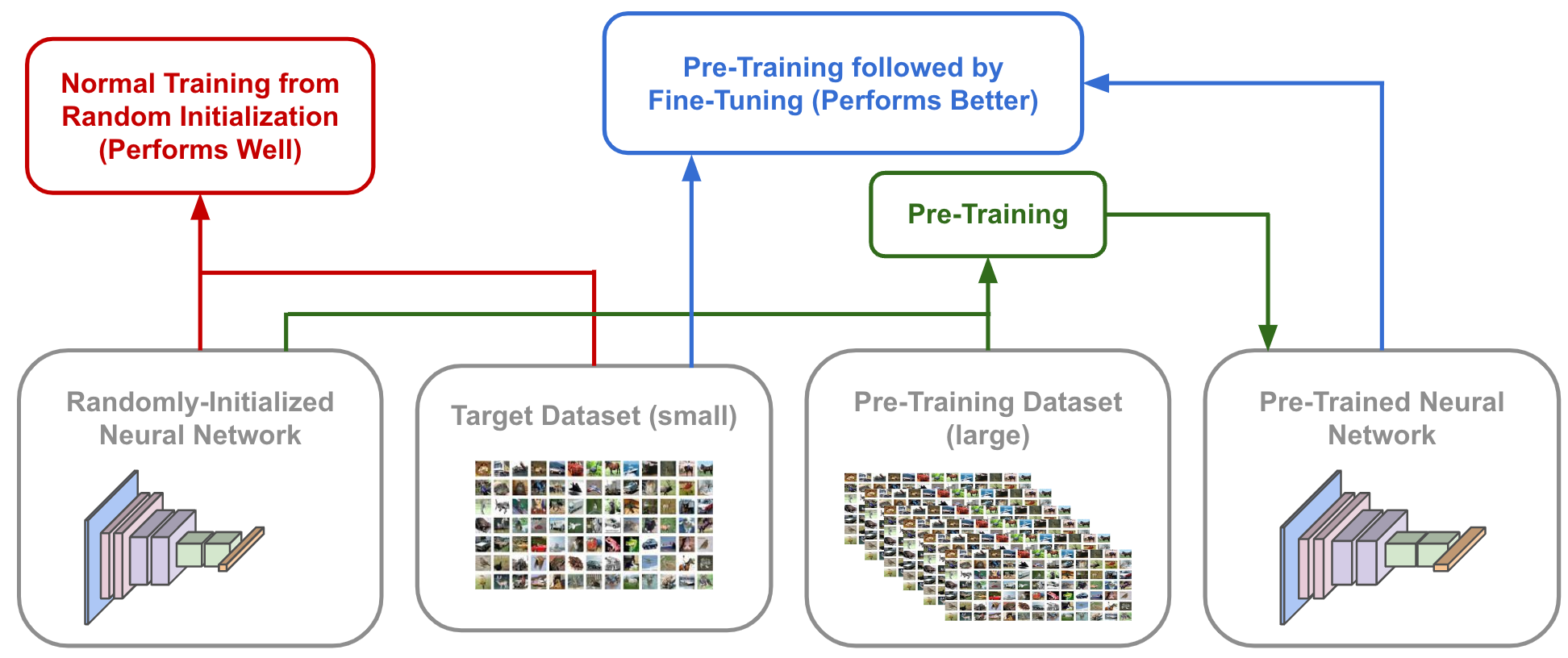
Illustration of the Differences between Pre-Training, Fine-Tuning, and Normal Training of a Neural Network
Pre-trained model parameters are often used as a “warm start” for performing training on other datasets, often referred to as the downstream or target dataset. Instead of initializing model parameters randomly when performing downstream training, we can set model parameters equal to the pre-trained weights and fine-tune—or further train—these weights on the downstream dataset; see the figure above. If the pre-training dataset is sufficiently large, such an approach yields improved performance, as the model learns concepts when pre-trained on the larger dataset that cannot be learned using the target dataset alone.
Publications
Within the following overviews, I will discuss several papers that demonstrate the existence of critical learning periods within deep neural networks. The first paper studies the impact of data blurring on the learning process, while the following papers study learning behavior with respect to model regularization and data distributions during training. Despite taking different approaches, each of these works follow a similar approach of:
Applying some impairment to a portion of the learning process
Analyzing how such a deficit impacts model performance after training
Critical Learning Periods in Deep Networks [1]

Main Idea. This study, performed by a mixture of deep learning and neuroscience experts, explores the connection between critical learning periods in biological and artificial neural networks. Namely, authors find that introducing a deficit (e.g., blurring of images) to the training of deep neural networks, even for only a short period of time, can result in degraded performance. Going further, the extent of the damage to performance depends on when and how long the impairment is implied—a finding that mirrors the behavior of biological systems.
For example, if the impairment is applied at the beginning of training, there exists a sufficient number of impaired learning epochs, beyond which the deep network’s performance will never recover. Biological neural networks demonstrate similar properties with respect to early impairments to learning. Namely, experiencing an impairment to learning for too long during early stages of development can have permanent consequences (e.g., amblyopia). The figure above demonstrates the impact of critical learning periods in both artificial and biological systems.
At a high level, the discovery within this paper can be simply stated as follows:
If one impairs a deep network’s training process in a sustained fashion during the early epochs of training, the network’s performance cannot recover from this impairment
To better understand this phenomenon, authors quantitatively study the connectivity of the network’s weight matrices, finding that learning is comprised of a two-step process of “memorizing”, then “forgetting”. More specifically, the network memorizes data during the early learning period, then reorganizes/forgets such data as it begins to learn more efficient, generalizable patterns. During the early memorization period, the network navigates a bottleneck in the loss landscape—the network is quite sensitive to learning impairments as it traverses this narrow landscape. Eventually, however, the network escapes this bottleneck to discover a wider valley that contains many high-performing solutions—the network is more robust to learning impairments within this region.
Methodology. Within this work, authors train a convolutional neural network architecture on the CIFAR-10 dataset. To mimic a learning impairment, images within the dataset are blurred for varying numbers of epochs at different points during the learning process. Then, the impact of this impairment is measured via the model’s test accuracy after the full training process has been completed. Notably, the learning impairment is typically only applied during a small portion of the full learning process. By studying the impact of such impairments on network performance, the authors discover that:
If the impairment is not removed sufficiently early during training, then network performance will be permanently damaged.
Sensitivity to such learning impairments peaks during the early period of learning (i.e., the first 20% of epochs).
To further explore the properties of critical learning periods in deep networks, authors measure the Fisher information within the model’s parameters, which quantitatively describes the connectivity between network layers, or the amount of “useful information” contained within network weights.
Fisher information is found to increase rapidly during early training stages, then decay throughout the remainder of training. Such a trend reveals that the model first memorizes information during the early learning phase, then slowly reorganizes or reduces this information—even as classification performance improves—by removing redundancy and establishing robustness to non-relevant variability in the data. When an impairment is applied, the Fisher Information grows and remains much higher than normal, even after the deficit is removed, revealing that the network is less capable of learning generalizable data representations in this case. See the figure below for an illustration of this trend.

Findings.
Network performance is most sensitive to impairments during the early stage of training. If image blurring is not removed within the first 25-40% of training epochs (i.e., the exact ratio depends on network architecture and training hyperparameters) for the deep network, then network performance will be permanently damaged.
High-level changes to data (e..g, vertical flipping of images, permutation of output labels) do not have any impact of network performance. Additionally, performing impaired training with white noise does not damage network performance—completely sensory deprivation (i.e., this parallels dark rearing in biological systems) is not problematic to learning.
Pre-training may be detrimental to network performance if performed poorly (e.g., using images that are too blurry).
Fisher information is typically highest in the intermediate network layers, where low and mid-level image features can be most efficiently processed. Impairments to the learning process lead to a concentration of Fisher information in the final network layer, which contains no lower or mid-level features, unless the deficit is removed sufficiently early in training.
Time Matters in Regularizing Deep Networks: Weight Decay and Data Augmentation Affect Early Learning Dynamics, Matter Little Near Convergence [2]
Main Idea. The typical view of regularization (e.g., via weight decay or data augmentation) posits that regularization simply alters a network’s loss landscape as to bias the learning process towards final solutions with low curvature. The final, critical point of learning is smooth/flat in the loss landscape, which is (arguably) indicative of good generalization performance. Whether such an intuition is correct is a subject of hot debate—one can read several interesting articles about the connection between local curvature and generalization online.
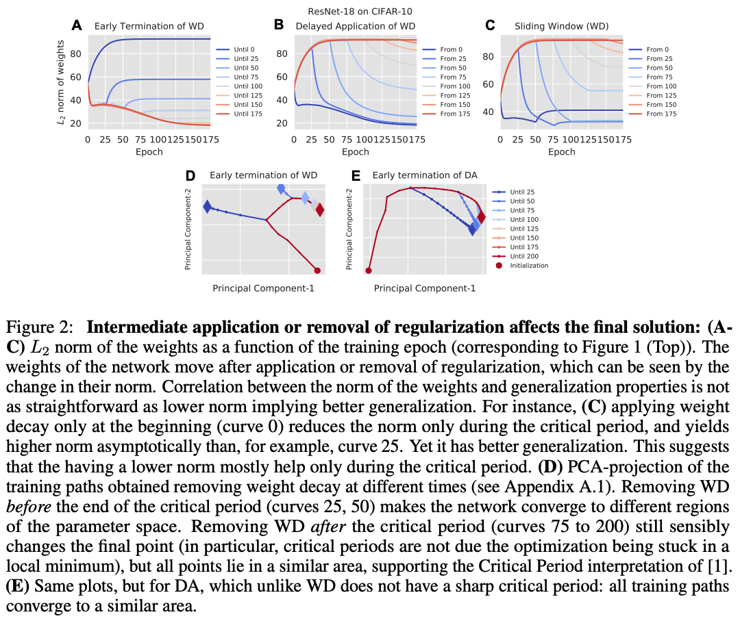
This paper proposes an alternative perspective of regularization, going beyond these basic intuitions. The authors find that removing regularization (i.e., weight decay and data augmentation) after the early epochs of training does not alter network performance. On the other hand, if regularization is only applied during the later stages of training, it does not benefit network performance—the network performs just as poorly as if regularization were never applied. Such results collectively demonstrate the existence of a critical period for regularizing deep networks that is indicative of final performance; see the figure above.
Such a result reveals that regularization does not simply bias network optimization towards final solutions that generalize well. If this intuition were correct, removing regularization during the later training periods—when the network begins to converge to its final solution—would be problematic. Rather, regularization is found to have an impact on the early learning transient, biasing the network optimization process towards regions of the loss landscape that contain numerous solutions with good generalization to be explored later in training.
Methodology. Similarly to previous work, the impact of regularization on network performance is studied using convolutional neural network architectures on the CIFAR-10 dataset. In each experiment, the authors apply regularization (i.e., weight decay and data augmentation) to the learning process for the first t epochs, then continue training without regularization. When comparing the generalization performance of networks with regularization applied for different durations at the beginning of training, authors find that good generalization can be achieved by only performing regularization during the earlier phase of training.
Beyond these initial experiments, the authors perform experiments in which regularization is only applied for varying durations at different points in training. Such experiments demonstrate the existence of a critical period for regularization. Namely, if regularization is applied only after some later epoch in training, then it yields no benefit in terms of final generalization performance. Such a result mirrors the findings in [1], as the lack of regularization imposed can be viewed as a form of learning deficit that impairs network performance.
Findings.
The effect of regularization on final performance is maximal during the initial, “critical” training epochs.
The critical period behavior of weight decay is more pronounced than that of data augmentation. Data augmentation impacts network performance similarly throughout training, while weight decay is most effective when applied during earlier epochs of training.
Performing regularization for the entire duration of training yields networks that achieve comparable generalization performance to those that only receive regularization during the early learning transient (i.e., first 50% of training epochs).
Using regularization or not during later training periods results in different points of convergence (i.e., the final solution is not identical), but the resulting generalization performance is the same. Such a result reveals that regularization “directs” training during the early period toward regions with multiple, different solutions that perform equally well.
On Warm-Starting Neural Network Training [3]

Main Idea. In real-world machine learning systems, it is common for new data to arrive in an incremental fashion. Generally, one will begin with some aggregated dataset, then over time, as new data becomes available, this dataset grows and evolves. In such a case, sequences of deep learning models are trained over each version of the dataset, where each model takes advantage of all the data that is available so far. Given such a setup, however, one may begin to wonder whether a “warm start” could be formulated, such that each model in this sequence begins training with the parameters of the previous model, mimicking a form of pre-training that allows model training to be more efficient and high-performing.
In [3], the authors find that simply initializing model parameters with the parameters of a previously-trained model is not sufficient to achieve good generalization performance. Although final training losses are similar, models that first pre-trained over a smaller subset of data, then fine-tuned on the full dataset achieve degraded test accuracy in comparison to models that are randomly initialized and trained using the full dataset. Such a finding mimics the behavior of critical learning periods outlined in [1, 2]—the early phase of training is completely focused upon a smaller data subset (i.e., the version of the dataset before the arrival of new data), which results in degraded performance once the model is exposed to the full dataset. However, the authors propose a simple warm-starting technique that can be used to avoid such deteriorations in test accuracy.
Methodology. Consider a setup where new data arrives into a system once each day. In such a system, one would ideally re-train their model when this new data arrives each day. Then, to minimize training time, a naive warm starting approach could be implemented by initializing the new model’s parameters with the parameters of the previous days’ model prior to training/fine-tuning. Interestingly, however, such a warm starting approach is found to yield models that generalize poorly, revealing that pre-training over an incomplete subset of data is a form of learning impairment when applied during a critical period.
To overcome the impact of this impairment, the authors propose a simple technique called Shrink, Perturb, Repeat that:
Shrinks model weights towards zero.
Adds a small amount of noise to model weights.
If such a procedure is applied to the weights of a previous model trained over an incomplete subset of data, then the parameters of this model can be used to warm start training over the full dataset without causing any deterioration in generalization performance. Although the amount of shrinking and scale of the noise introduce new hyperparameters to the training process, this simple trick yields remarkable computational savings—due to the ability to warm start, and thus speed up, model training—with no deterioration to network performance.
To elucidate the efficacy of this approach, authors explain that a naive warm start methodology experiences significant imbalances between the gradients of new and old data. Such imbalances are known to negatively impact the learning process [4]. However, shrinking and noising model parameters prior to training both (i) preserves network predictions and (ii) balances the gradient contributions of new and old data, thus striking a balance between leveraging previously-learned information and adapting to newly-arriving data.
Findings.
Although critical learning periods associated with incomplete datasets are demonstrated in deep networks, simpler models (e.g., logistic regression) do not experience such an effect (i.e., likely because training is convex).
The degradation in test accuracy due to naive warm starting cannot be alleviated via tuning of hyperparameters like batch size or learning rate.
Only a small amount of training (i.e., a few epochs) over an incomplete subset of data is necessary to damage the test accuracy of a model trained over the full dataset, further revealing that training over incomplete data is a form of learning impairment with connections to critical learning periods.
Leveraging the Shrink, Perturb, Repeat method completely eliminates the generalization gap between randomly-initialized and warm-started models, enabling significant computational savings.
Is deep learning theory missing the mark?
The existence of critical learning periods gives birth to an interesting perspective of the learning process for deep neural networks. Namely, the fact that such networks cannot recover from impairments applied during the early epochs of training reveals that learning progresses in two, distinct phases, each of which have interesting properties and behavior.
Critical Learning Period: the memorization period. The network must navigate a narrow/bottlenecked region of the loss landscape.
Converging to a Final Solution: the forgetting period. After traversing a bottlenecked region of the loss landscape, the network enters a wide valley of many equally-performant solutions to which it can converge.
The critical learning period during the early learning transient plays a key role in determining final network performance. Later changes to the learning process cannot alleviate mistakes during this early period.
Interestingly, most theoretical work in the domain of deep learning is asymptotic in nature. Put simply, this means that such methods of analysis focus upon the properties of the final, converged solution after many iterations of training. No notion of critical learning periods or different phases of learning appear. The convincing empirical results that outline the existence of critical learning periods within deep networks hint that there is more to deep learning than is revealed by current, asymptotic analysis. Theoretical analysis that truly captures the complexity of learning within deep networks is yet to come.
Takeaways
The takeaways from the overview can be stated pretty simply:
Neural network training seems to proceed in two major phases—memorization and forgetting.
Impairing the learning process during the first, early phase is not good.
To be a bit more specific, learning impairments during the first phase aren’t just bad… they are seemingly catastrophic. One cannot recover from these impairments during the second phase, and the resulting network is doomed to poor performance in most cases. The work overviewed here has demonstrated this property in numerous domains, showing that the following impairments applied during the first phase of learning can degrade network generalization:
Sufficiently blurred images
Lack of regularization (i.e., data augmentation or weight decay)
Lack of sufficient data
Critical learning periods provide a unique perspective on neural network training that makes even seasoned researchers question their intuitions. This two-phase view of neural network training defies commonly-held beliefs and is not reflected within much of the theoretical analysis of deep networks, revealing that much more work is to be done if we are to collectively arrive at a more nuanced understanding of deep learning. With this in mind, one may begin to wonder whether the most fundamental breakthroughs in our understanding of deep networks are yet to come.
Further Reading
Friendly Training: Neural Networks Can Adapt Data To Make Learning Easier
Catastrophic Fisher Explosion: Early Phase Fisher Matrix Impacts Generalization
New to the Newsletter?
Hello! I am Cameron R. Wolfe, a research scientist at Alegion and PhD student at Rice University studying the empirical and theoretical foundations of deep learning. This is the Deep (Learning) Focus newsletter, where I pick a single, bi-weekly topic in deep learning research, provide an understanding of relevant background information, then overview a handful of popular papers on the topic. If you like this newsletter, please subscribe or check out my other writings!
I end each newsletter with a quote to ponder. I’m a big fan of stoicism, deep focus, and finding passion in life. So, finding this quote each week keeps me accountable with my reading, thinking, and mindfulness. I hope you enjoy it!
“One day, in retrospect, the years of struggle will strike you as the most beautiful.”
-Sigmund Freud
Keep learning and don’t forget to have some fun along the way!
Bibliography
[1] Achille, Alessandro, Matteo Rovere, and Stefano Soatto. "Critical learning periods in deep networks." International Conference on Learning Representations. 2018.
[2] Golatkar, Aditya Sharad, Alessandro Achille, and Stefano Soatto. "Time matters in regularizing deep networks: Weight decay and data augmentation affect early learning dynamics, matter little near convergence." Advances in Neural Information Processing Systems 32 (2019).
[3] Ash, Jordan, and Ryan P. Adams. "On warm-starting neural network training." Advances in Neural Information Processing Systems 33 (2020): 3884-3894.
[4] Yu, Tianhe, et al. "Gradient surgery for multi-task learning." Advances in Neural Information Processing Systems 33 (2020): 5824-5836.
[5] Eric R Kandel, James H Schwartz, Thomas M Jessell, Steven A Siegelbaum, and A James Hudspeth. Principles of Neural Science. McGraw-Hill, New York, NY, 5th edition, 2013.